Agroforestry Image

Use of mixture designs and models for agroforestry

Abstract

Agroforestry systems by their very mature are complex but are found promoted for many ecological and socio-economic benefits. Experimentation with such systems also inherits many of these complexities. Other than the regular design and analytical options available, the system throws in challenges in the analyses primarily because of varied nature of response variables. Mixture designs and models are especially suited for experimenting with agroforestry systems the latter being mixtures of multiple components. This presentation explores the possibilities of using some of mixture designs and related analytical techniques in conducting agroforestry experiments after a preamble of standard design and analytical methods used in forestry/ agriculture.

Introduction

Agroforestry is a collective name for land-use systems and technologies where woody perennials are grown on the same land-management units as agricultural crops and/or animals, in some form of spatial arrangement or temporal sequence. Nair (~2000) notes that from a purely ecological point, certain types of systems can be identified as characteristic of each major ecological region and lists out the following examples.

Humid/subhumid lowlands – home gardens, plantation crop combinations, multilayer tree gardens, alley cropping and other intercropping systems.

Semi-arid/arid lands– silvipastoral systems, windbreaks/shelter belts, MPTs for fuel/fodder, MPTs on farmlands.

Highlands– soil conservation hedges, silvipastoral combinations, plantation crop systems.

The definition above implies that an agroforestry system normally involves two or more species of plants, at least one of which is a woody perennial, always has two or more outputs, and has the cycle of more than one year. Obviously, there is scope for much inter-component interactions in such systems, positive and/or negative. The system thus is more complex than monocropping and would require special ways of handling these characteristics in respect of design and analysis of experiments. Although the basics of experimentation such as randomization, replication and local control remain the same and many standard designs are applicable with such systems, certain modifications are suggestive to take care of the specialties involved. Hence the standard methodology is described first followed by some special modes of investigations with agroforestry systems.

Standard design and analytical models

The regular designs used for field experiments like randomized complete block design (RCBD), split-plot design and strip-plot design are useful in many situations with agroforestry trials and their use is governed by the particular tree-crop combination under consideration. With large number of factors and levels, fractional factorials or confounded designs come to be of use. Certain systematic designs like fan designs are found suggested for spacing trials to avoid the adjacent occurrence of high and low intensity spacing levels. However, they have their limitations due to lack of randomization of the levels. In all cases, appropriate plot size, block size and borders have to be chosen to enable control of heterogeneity and to avoid edge effects. Subsampling within plots will be required where complete enumeration is not possible within a particular plot.

Characterizing the treatments is of prime importance in agroforestry. The proportion of area occupied by each crop in the mixture at the time of planting is a direct measure in this regard. For instance, a 1:1 mixture could indicate half the area planted under each crop initially. Because the produce from agroforestry systems is of varied nature, they have to be brought to a common ground for any comparison between the treatments. Land Equivalent Ratio (FAO, 1985) is one such index which will show the land area in the system that would be required to produce the same yields as one hectare of intercropping. For a scenario where a total of m crops is intercropped, the land equivalent ratio LER can be calculated as

where m is the number of different crops intercropped, IYi is the yield for i th the crop under intercropping, and SYi is the yield for the i th crop under a sole-crop regime on the same area. For the case of just two crops, the situation could be as follows.

In similar lines, the total biomass per unit area, combined economic returns per unit area are summative measures that can be considered as response variables. The analysis would involve analysis of variance (ANOVA) or analysis of covariance (ANACOV) followed by pairwise comparison or testing of contrasts. The other option is to go for multivariate ANOVA or ANACOV wherein the identity of individual components is retained. The combined analysis takes the form of MANOVA followed by tests based on Hotelling’s T2.

Repeated measurements over time could be a cardinal feature of agroforestry systems for which the analysis would utilize repeated measures model giving information on treatments, the time factor and treatment by time interaction. When several characteristics are involved, it would be better to resort to dimension reduction techniques like principal components analysis followed by ANOVA of the principal components. Agroforestry systems do not generally involve large number of treatments and so may not invoke multiplicity issues in treatment comparisons. One other source of data is that coming from groups of experiments or multilocation trials. The important question here is about the genotype by environment interaction. The same agroforestry system when tried in different soil/climatic zones may behave differently and such information is to be gainfully used. So is the case when several independent investigations are undertaken with similar or different tree-crop combinations. Network meta-analysis will go a long way in synthesizing information from such data sources.

Mixture designs

One grand design proposition for experiments with agroforestry systems is that based on mixture models. A mixture experiment involves mixing various proportions of two or more components to make different compositions of an end product. Mixture components proportions xi are subject to the constraints,

(1)

where q is the number of components. As a result, the factor space reduces to regular (q-1) dimensional simplex Sq-1. For q=2 it is a straight line x1+x2=1 and for q=3 it is an equilateral triangle. One related question is how to compute the proportions under different crops in an agroforestry system. The one based on planted area seems to qualify for the same.

Scheffe (1958, 1963) introduced the {q,m} simplex lattice designs and simplex-centroid designs. The {q,m} simplex lattice designs are characterized by the symmetric arrangements of points within the experimental region and a well-chosen polynomial equation to represent the response surface over the entire simplex region. The polynomial has exactly as many parameters as there are number of points in the associated simplex lattice design.

The {q,m} simplex lattice design given by Scheffe (1958) consists of q+m-1Cm points where each component proportion takes (m+1) equally spaced values xi=0,1/m, 2/m,…,1; i=1,2,…,q, ranging between 0 and 1 and all possible mixtures with these component proportions are used.

For example: a {3,2} simplex lattice will consist of 3+2-1C2 i.e. 4C2=6 points. Each xi can take m+1=3 possible values xi=0, 1⁄2,1 with which the possible design points are (1,0,0), (0,1,0), (0,0,1), (1⁄2, 1⁄2, 0), (0, 1⁄2, 1⁄2), (1⁄2, 0, 1⁄2).

Scheffe (1963) gave simplex centroid designs which consists of 2q -1 points with q permutations of (1,0,0,…, 0) (i.e., q pure blends), (qC2) permutations of (1⁄2,1⁄2,0,…0) (i.e. (qC2) binary blends),…, and the overall centroid (1/q, 1/q,…, 1/q) (i.e. the q-nary blend).

For q=3, the simplex centroid design consists of seven points (1,0,0), (0,1,0), (0,0,1), (1⁄2, 1⁄2, 0), (0, 1⁄2, 1⁄2), (1⁄2, 0, 1⁄2) and (1/3,1/3,1/3).

The (q,m} simplex-lattice and q-component simplex-centroid designs are boundary designs in that, with the exception of the overall centroid, the points of these designs are positioned on the boundaries (vertices, edges, faces, etc.) of the simplex factor space. Axial designs on the other hand, are designed to consist mainly of complete mixture or q-component blends where most of the points are positioned inside the simplex. Axial designs have been recommended for use when component effects are to be measured and in screening experiments, particularly when first-degree models are to be fitted. Designs with points lying on the axis of components, that is imaginary line extending the base points xi=0, xj=1/(q-1) v i≠j to the vertex where xi=1, xj=0 v i≠j, are called axial designs.

Mixture models

Data from mixture designs are analyzed through mixture models involving Scheffe’s canonical polynomials. Scheffe (1958) introduced canonical polynomials to be used with his simplex lattice designs. These polynomials are obtained by modifying the usual polynomial model in xi by using the restriction Σxi=1.

The number of terms in {q,m} polynomial or canonical polynomial is (q+m-1Cm) and this number is equal to the number of points that make up the associated {q,m} simplex lattice design. For example, for m=1 the linear canonical model is

η = ∑ βixi

(2)

The number of terms in equation (2) is q, which is the number of points in the {q,1} lattice. For m=2, the second-degree canonical polynomial is

η = ∑ βixi + ∑∑ βijxixj

(3)

The number of terms in (1.3) is q+q(q-1) /2 = q(q+1) /2.

The full cubic canonical polynomial or (q,3) polynomial is

(4)

A simpler formula for a special case of the cubic polynomial is the special cubic polynomial

(5)

the number of terms in equation (5) is q(q2 + 5)/6.

For each of the above models, formulae for estimating the parameters and their variances are available in Cornell (2002).

The analysis of variance table takes the regular form of a regression model:

Source of Variation Degrees of Freedom Sum of Squares Mean squares
Regression (fitted model) p-1 MSR=SSR/(p-1)
Residual N-p MSE=SSE/(N-p)
Total N-1

The results of mixture experiments are usually depicted in the form of a contour plot which shows the intensity of response across the factor space. The following graph shows the CO2 adsorption rates for MCM-41 synthesized using three types of surfactants (Costa et al, 2015). The optimal mixture has been C17: C19 in equal proportion giving a CO2 adsorption rate of 0.62 g CO2/g adsorbent.

Process variables

In some mixture experiments, the response depends not only on the proportion of the components present in the mixture but also on the processing conditions. Process variables are factors in an experiment that do not form any portion of the mixture but whose levels when changed could affect the blending properties of the ingredients. The models involve both mixture variables and process variables. For instance, in agroforestry experiments, the same mixture could occur at different planting densities or fertilizer levels.

The methodology used to construct mixture designs involving process variables is composition of two smaller designs, one being a mixture designs for the mixture components only and the other being factorial/fractional factorial design for the process variables. For example, with two mixture components having the proportions x1 and x2, suppose there are also two process variables, denoted by z1 and z2 and each process variable is to be studied at two levels. If a three-term quadratic model in x1 and x2 is to be fitted to data collected at the point of a {2,2} simplex lattice, the combined {2,2} lattice x 22 factorial arrangement can be used.

For instance, the three terms quadratic model in two components

(6)

when combined with the four-term main and interaction effect model in z1 and z1

(7)

produces the 12-term combined model

(8)

where

(9)

These models help us also understand the interactions between process variables and mixture components.

Conclusions

Considerable developments have taken place in this field and it is open for agroforestry researchers to adopt a suitable design and analytical technique for his/her studies. However, the real advantage of mixture models is, having tried a few pure or combination mixtures in reality, the models have the capability to predict the responses associated with any level of mixing across the range experimentation or factor space.


biodiversity

Modified Shannon index of biodiversity

Shannon-Wiener index or Shannon index is an established measure of biodiversity in ecological studies. It is a measure of relative abundance of a set of organisms defined by,

(1)

where pi is the proportion of i th species in the community

ln indicates logarithm

Shannon index increases as the number of species classes increases, or the proportional distribution among species types become more equitable. For a given number of species classes, the maximum value of the Shannon index is reached when all classes have the same proportion. The logarithm is conventionally taken to the base two, but of late, natural logarithm is admitted.

This index, although efficient, has a significant deficiency. Suppose two plots have the same number of species with the same relative abundances (pi ). Shannon’s index will return the same value for H, indicating that the two plots are equally diverse. However, if the first plot contains species each from a different family and in the other plot, all the species are from the same family, the more diverse state of the first plot does not get reflected in the Shannon’s measure. Hence this index needs to be modified. Some proposals are made here, with illustrations. An extension of the Shannon index up to the family level is presented here.

(2)

where pi is the proportion of i th species in the community

gi is the proportion of i th genus in the community

fi is the proportion of i th family in the community

s, g, f indicate the number of species, number genera, and number of families respectively

ln indicates logarithm

There is no problem with scaling here as all the components individually are based on proportions that add up to unity.

Equation (2) can more tersely be expressed as

H = Hs + Hg + Hf

(3)

The situation is described using an artificial set of data for two plots (Table 1). The first site contains 12 species belonging to 6 genera and two families. The second site includes 12 species belonging to a single genus of a single family. The number of individuals 1under each group is taken as 10 for convenience. The different components of the modified index are presented in the last column.

In the first plot, the overall index is almost double that of the second plot because of the higher genus and family diversity. The basic measure of species diversity (Hs) remains the same for the two plots. It is important to consider this aspect of diversity in all future studies in ecology.

Status of two plots using artificial data:
Site Family Genus Species Abun
-dance
Index
1 F1 F1G1 F1G1S1 10
1 F1 F1G1 F1G1S2 10
1 F1 F1G2 F1G2S1 10
1 F1 F1G2 F1G2S2 10
1 F1 F1G3 F1G3S1 10
1 F1 F1G3 F1G3S2 10
1 F2 F2G1 F2G1S1 10
1 F2 F2G1 F2G1S2 10
1 F2 F2G2 F2G2S1 10
1 F2 F2G2 F2G2S2 10 Hs = 2.48
1 F2 F2G3 F2G3S1 10 Hg = 1.79
1 F2 F2G3 F2G3S2 10 Hf = 0.69
H’ = 4.96
2 F1 F1G1 F1G1S1 10
2 F1 F1G1 F1G1S2 10
2 F1 F1G1 F1G1S3 10
2 F1 F1G1 F1G1S2 10
2 F1 F1G1 F1G1S4 10
2 F1 F1G1 F1G1S5 10
2 F1 F1G1 F1G1S6 10
2 F1 F1G1 F1G1S7 10
2 F1 F1G1 F1G1S8 10
2 F1 F1G1 F1G1S9 10
2 F1 F1G1 F1G1S10 10 Hs = 2.48
2 F1 F1G1 F1G1S11 10 Hg = 0
2 F1 F1G1 F1G1S12 10 Hf = 0
H = 2.48

meta

Use of Meta-Analysis in Research

Science is a cumulative process. Therefore, it is not surprising that one can often find multiple studies addressing the same basic question. Researches trying to aggregate and synthesize the literature on a particular topic are increasingly conducting meta-analyses. Broadly speaking, a meta-analysis can be defined as a systematic literature review supported by statistical methods where the goal is to aggregate and contrast the findings from several related studies. For instance, in medical research, meta-analysis aims to assess the relative effectiveness of several interventions and synthesize evidence across a network of randomized and/or non-randomized clinical trials or other relevant sources of information. For example, we may be able to express the results from a randomized clinical trial examining the effectiveness of a medication in terms of an odds ratio, indicating how much higher/lower the odds of a particular outcome (e.g., remission) were in the treatment compared to the control group. The set of odds ratios from several studies examining the same medication then forms the data which is used for further analyses. For example, we can estimate the average effectiveness of the medication (i.e., the average odds ratio) or conduct a moderator analysis, that is, we can examine whether the effectiveness of the medication depends on the characteristics of the studies like average age of the participants, geographical location etc. Depending on the types of studies and the information provided therein, a variety of different outcome measures can be used for a meta-analysis, including the odds ratio, relative risk, risk difference, the correlation coefficient, and the (standardized) mean difference.

Both fixed and random/mixed effects models are employed to analyze the data from meta-analytical studies. Also, the models work both under frequentist and Bayesian framework. Bayesian analysis will require specification of priors, i.e., information available on the status of parameters of our model. A graphical overview of the synthesized results can be obtained by creating a forest plot. The following figure shows the relative risk of a tuberculosis infection in the treated versus the control group with corresponding 95% confidence intervals in the individual studies based on a random effects model. The mean effect is usually indicated in the shape of a diamond at the bottom.

Network meta-analysis (NMA) extends traditional meta-analysis concept by including multiple pairwise comparisons across a range of interventions across studies. With a network meta-analysis, the relative effectiveness of two treatments can be estimated even if no studies directly compare them (indirect comparisons). It provides direct evidence which comes from studies directly randomizing treatments of interest and indirect evidence which comes from studies comparing treatments of interest with a common comparator. Direct and indirect treatment comparisons are also popularly referred to as mixed treatment comparisons (MTC). For instance, with two independent trials with treatments H and Q against Placebo (P), it is possible to make indirect comparisons between H and Q based on NMA. If a direct comparison between H and Q is available, this information can then be combined with indirect comparison to produce stronger evidence.

NMA involves certain assumptions like the following:
  • Similarity: Clinical and methodological homogeneity with respect to effect modifiers.
  • Transitivity: Requires that sets of ABdirect and BCdirect studies are similar in distributions of effect modifiers, for a valid indirect comparison (say ACindirect).
  • Consistency: Occurs when subtraction equation, (ACindirect = ABdirect – BCdirect) is supported by the data. Inconsistency: Refers to the degree of disagreement between source specific treatment effects (e.g., moderate vs severe illness) and is measured by the difference between direct and indirect estimates (ACdirect – ACindirect ) beyond what can be explained by chance.
  • Heterogeneity: Refers to the degree of disagreement between study-specific treatment effects beyond what is explained by chance variability.

We can see the overall structure of treatment comparisons in our network through a netgraph. We can see that the edges have a different thickness, which corresponds to how often we find this specific comparison in our network. We see that Rosiglitazone has been compared to Placebo in many trials (Note: short names are used in the graph). We also see the one multi-arm trial in our network, which is represented by the blue triangle in our network. This is the study Willms2003, which compared Meformin, Acarbose and Placebo.

The estimates of direct and indirect evidence could be of the following form.

comparison k prop nma direct indir Diff z p-value
acar:benf 0 0 -0.1106 -0.1106
acar:metf 1 0.28 0.2850 0.2000 0.3182 -0.1182 -0.21 0.8368
acar:migl 0 0 0.1079 0.1079
acar:piog 0 0 0.2873 0.2873
acar:plac 2 0.65 -0.8418 -0.8567 -0.8138 -0.0429 -0.08 0.9338
acar:rosi 0 0 0.3917 0.3917
acar:sita 0 0 -0.2718 -0.2718
acar:sulf 1 0.53 -0.4252 -0.4000 -0.4538 0.0538 0.10 0.9194
acar:vild 0 0 -0.1418 -0.1418
Legend:

comparison – Treatment comparison

k – Number of studies providing direct evidence

prop – Direct evidence proportion

nma – Estimated treatment effect (MD) in network meta-analysis

direct – Estimated treatment effect (MD) derived from direct evidence

indir – Estimated treatment effect (MD) derived from indirect evidence

Diff – Difference between direct and indirect treatment estimates

z – z-value of test for disagreement (direct versus indirect)

p-value – p-value of test for disagreement (direct versus indirect)

The important information here is in the P-value column. If the value in this column is P<0.05, there is a significant disagreement (inconsistency) between the direct and indirect estimate. We see in the output that there are indeed a few comparisons showing significant inconsistency between direct and indirect evidence when using the random effects model.

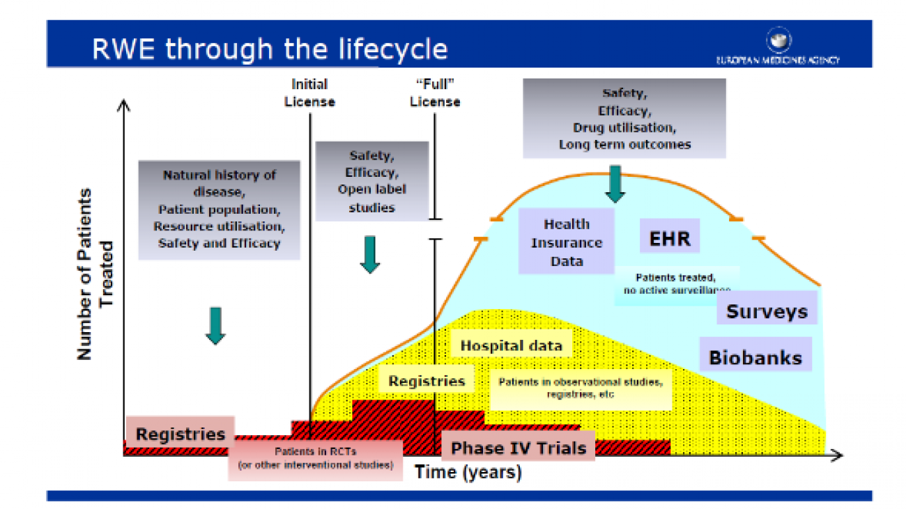
Researchers are also increasingly using real world evidence (RWE) for synthesizing information from nonclinical sources with information from regular randomized clinical trials (RCT). Real world evidence (RWE) can include non-randomized studies, electronic health records, disease registries, and claims data but are not limited to these. Although RCTs are considered the most reliable source of information on relative treatment effects, their strictly experimental setting and inclusion criteria may limit their ability to predict results in real-world clinical practice. RWE is increasingly used due to its greater potential for generalizability to clinical practice than RCT findings. However, RWE is associated with selection bias due to the absence of randomization. The transition of findings from RCT towards RWE is depicted in the following figure.

FDA recognizes Real-World Data (RWD) as data relating to patient health status and/or the delivery of health care routinely collected from a variety of sources. The reliability of RWD, RWD sources, and resultant analyses are assessed by evaluating several factors as how the data were collected and that data quality and integrity are sufficient (data assurance).

With respect to analyzing the RWE data, all the methods of NMA can be utilized to both analyze and integrate with data from randomized clinical trials provided we have an initial estimate of the treatment effect and its variance from each individual source of evidence.

Test-tubes with blue liquids over business document

Role of Statistics in Scientific Research

Research in science uses scientific method which is popularly known as the inductive-deductive approach. Scientific method entails formulation of hypotheses from observed facts followed by deductions and verifications repeated in a cyclical process. Facts are observations which are taken to be true. Hypothesis is a tentative conjecture regarding the phenomenon under consideration. Deductions are made out of the hypotheses through logical arguments which in turn are verified through objective methods. The process of verification may lead to further hypotheses, deductions and verification in a long chain in the course of which scientific theories, principles and laws emerge.

As a case of illustration, we may consider Edward Jenner’s trials with smallpox. He observed that people who have had cowpox do not become ill with smallpox from which he hypothesized that cowpox must be giving immunity against smallpox. The deduction he made was that if a person is intentionally infected with cowpox, then that person will be protected from becoming ill after a purposeful exposure to smallpox. Later this was verified by infecting people with cowpox followed by infecting with smallpox. This trial led to the conclusion that infecting a person with cowpox protects from infection with smallpox.

The two main features of scientific method are its repeatability and objectivity. Although this is rigorously achieved in the case of many physical processes, biological phenomena are characterised by variation and uncertainty. Experiments when repeated under similar conditions need not yield identical results, being subjected to fluctuations of random nature. Also, observations on the complete set of individuals in the population are out of question many times and inference may have to be made quite often from a sample set of observations. The science of statistics is helpful in objectively selecting a sample, in making valid generalisations out of the sample set of observations and also in quantifying the degree of uncertainty in the conclusions made.

Two major practical aspects of scientific investigations are collection of data and interpretation of the collected data. The data may be generated through a sample survey on a naturally existing population or a designed experiment on a hypothetical population. The collected data are condensed and useful information extracted through techniques of statistical inference. This apart, a method of considerable importance which has gained wider acceptance in recent times with the advent of computers is simulation. This is particularly useful because simulation techniques can replace large scale field experiments which are extremely costly and time consuming. Mathematical models are developed which capture most of the relevant features of the system under consideration after which experiments are conducted in computer rather than with real life systems.

In a broad sense, all in situ studies involving non-interfering observations on nature can be classed as surveys. These may be undertaken for a variety of reasons like estimation of population parameters, comparison of different populations, study of the distribution pattern of organisms or for finding out the interrelations among several variables. Observed relationships from such studies are not many times causative but will have predictive value. Studies in sciences like economics, ecology and wildlife biology generally belong to this category. Statistical theory of surveys relies on random sampling which assigns known probability of selection for each sampling unit in the population.

Experiments serve to test hypotheses under controlled conditions. Experiments are conducted with pre-identified treatments on well-defined experimental units. The basic principles of experimentation are randomization, replication and local control which are the prerequisites for obtaining a valid estimate of error and for reducing its magnitude. Random allocation of the experimental units to the different treatments ensures objectivity, replication of the observations increases the reliability of the conclusions and the principle of local control reduces the effect of extraneous factors on the treatment comparison.

Experimenting on the state of a system with a model over time is termed simulation. A system can be formally defined as a set of elements also called components. The elements (components) have certain characteristics or attributes and these attributes have numerical or logical values. Among the elements, relationships exist and consequently, the elements are interacting. The state of a system is determined by the numerical or logical values of the attributes of the system elements. The interrelations among the elements of a system are expressible through mathematical equations and thus the state of the system under alternative conditions is predictable through mathematical models. Simulation amounts to tracing the time path of a system under different conditions.

While surveys and experiments and simulations are essential elements of any scientific research programme, they need to be embedded in some larger and more strategic framework if the programme as a whole is to be both efficient and effective. Increasingly, it has come to be recognized that systems analysis provides such a framework, designed to help decision makers to choose a desirable course of action or to predict the outcome of one or more courses of action that seems desirable. A more formal definition of systems analysis is the orderly and logical organisation of data and information into models followed by rigorous testing and exploration of these models necessary for their validation and improvement.

Research related to biology extends from molecular level to the whole of biosphere. The nature of the material dealt with largely determines the methods employed for making investigations. Many levels of organization in the natural hierarchy such as micro-organisms or human beings are amenable to experimentation but only passive observations and modelling are possible at certain other levels. Regardless of the objects dealt with, the logical framework of the scientific approach and the statistical inference can be seen to remain the same.

Modern scientific research has witnessed large paradigm shifts with the availability of huge datasets, increased computational power and discovery of complex algorithms leading to machine learning. This change has happened right from the DNA level to areal mapping of vast landscapes. This has brought the science of statistics to the larger framework of data science, a combination of statistics, programming and domain knowledge. The inferential base of traditional fiducial statistics also got increasingly replaced by Bayesian methods which being computationally intensive were at the backstage so far. In short, we are witnessing revolutionary changes in the way knowledge discovery process happens!